2D Cellular Automata

Anders Lindman

Penultimate Amazing
Joined
Sep 17, 2010
Messages
13,833
"A cellular automaton consists of a regular grid of cells, each in one of a finite number of states, such as on and off (in contrast to a coupled map lattice). The grid can be in any finite number of dimensions. For each cell, a set of cells called its neighborhood is defined relative to the specified cell. An initial state (time t=0) is selected by assigning a state for each cell. A new generation is created (advancing t by 1), according to some fixed rule (generally, a mathematical function) that determines the new state of each cell in terms of the current state of the cell and the states of the cells in its neighborhood." -- http://en.wikipedia.org/wiki/Cellular_automaton

One example of a 2D cellular automaton is Conway's Game of Life:
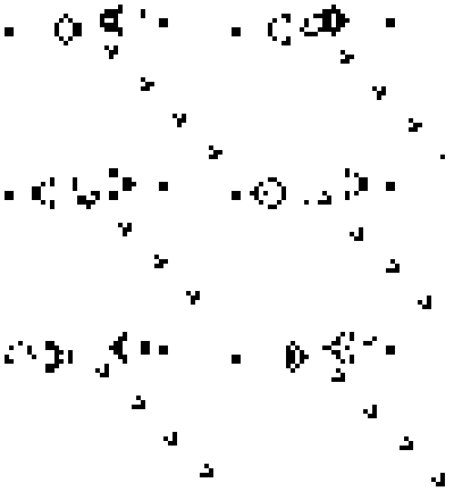
Gospers_glider_gun.gif


Instead of the cells having only an on or off value, each cell can be given an integer value, such as in this cellular automaton that produces a static pattern:

ca1.png


Source: http://jsfiddle.net/Hy3LY/

And here is another cellular automaton with integer values that produces a dynamic (moving) pattern:

ca2.png


Source (live demo): http://jsfiddle.net/eqUnv/
 
It's called emergent behaviour. Given the number of times you have been referred to it, I am surprised that it took you so long to latch on to it. Yet, as usual, you belatedly gather some facts but entirely miss the point.

Yawn.
 
It's called emergent behaviour. Given the number of times you have been referred to it, I am surprised that it took you so long to latch on to it. Yet, as usual, you belatedly gather some facts but entirely miss the point.

Yawn.

Stephen Wolfram has a concept he calls computational irreducibility that also applies.

"While many computations admit shortcuts that allow them to be performed more rapidly, others cannot be sped up. Computations that cannot be sped up by means of any shortcut are called computationally irreducible. The principle of computational irreducibility says that the only way to determine the answer to a computationally irreducible question is to perform, or simulate, the computation." -- http://mathworld.wolfram.com/ComputationalIrreducibility.html

Wolfram also explored possible cellular automata of different kinds and he found a simple 1D automaton he calls Rule 30 that produces a complex pattern.

"Rule 30 is a one-dimensional binary cellular automaton rule introduced by Stephen Wolfram in 1983.[2] Using Wolfram's classification scheme, Rule 30 is a Class III rule, displaying aperiodic, chaotic behaviour.

This rule is of particular interest because it produces complex, seemingly random patterns from simple, well-defined rules. Because of this, Wolfram believes that Rule 30, and cellular automata in general, are the key to understanding how simple rules produce complex structures and behaviour in nature." -- http://en.wikipedia.org/wiki/Rule_30
 
By chance, are computationally irreducible cellular automata related to the similar to the P vs NP problem?

Seems that any cellular automata which simulates a Turing Machine would be unable to efficiently solve any number computational problems which have no known polynomial solution, nor the whole host of problems for which no computable solution is known. On the plus side, at least you can simulate the Game of Life in Game of Life.

This rule is of particular interest because it produces complex, seemingly random patterns from simple, well-defined rules. Because of this, Wolfram believes that Rule 30, and cellular automata in general, are the key to understanding how simple rules produce complex structures and behaviour in nature." -- http://en.wikipedia.org/wiki/Rule_30
See also L-systems and Langton's Ant, which beautifully demonstrate the phenomenon of hiding infinite detail inside a finite number of very simple rules ^_^
 
Last edited:
Computational irriducibility has been proven, IIRC.

It's the core of my argument that time must exist and cannot be an illusion per some theories of physics.

We can indeed do said calculations, and get proven results, and this calculation is embedded in the reality of physics, and thus said calculation must have been performed and couldn't suddenly have come into existence already-completed as a static structure via some "short circuit" calculation.

i.e. you cannot get the results of such processes, which are all over the place, without actually going through the motions, which requires (some kind) of time.
 
Last edited:
By chance, are computationally irreducible cellular automata related to the similar to the P vs NP problem?

I don't know. Could be related.

"A universal cellular automaton is a cellular automaton which, like a Turing machine, exhibits universality. von Neumann proved that an automaton consisting of cells with four orthogonal neighbors and 29 possible states would be capable of simulating a Turing machine for some configuration of about 200000 cells (Gardner 1983, p. 227)." -- http://mathworld.wolfram.com/UniversalCellularAutomaton.html
 
Here are several similar automata that can be stepped through manually: http://jsfiddle.net/t2hXe/

The states for the cells are two-dimensional, where one dimension represents the pixel value and the other a value that is added at each iteration.
 
Anders Lindman said:
Stephen Wolfram has a concept he calls computational irreducibility that also applies.

"While many computations admit shortcuts that allow them to be performed more rapidly, others cannot be sped up. Computations that cannot be sped up by means of any shortcut are called computationally irreducible. The principle of computational irreducibility says that the only way to determine the answer to a computationally irreducible question is to perform, or simulate, the computation." -- http://mathworld.wolfram.com/Computa...ucibility.html

By chance, are computationally irreducible cellular automata related to the similar to the P vs NP problem?
Answering my own question, here's the paper which describes "computationally irreducible cellular automata[/url], and it appears the meaning was more straightforward than I first thought:

A cellular automata is "computationally irreducible" if its behavior is non-periodic and produce structures that "seem random" (subjective judgement). So that the state of the automata at N steps cannot be inferred without actually iterating through N steps of the automata.

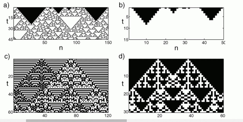
The paper goes a little further, explaining that a "computationally irreducible" automata has no computationally reducible "coarse graining", where coarse graining is a cellular automata whose "large scale behavior" can be modeled by a different set of rules. Here's a picture to illustrate:

coarsegraining_zps013a416e.gif


The rules of this automata allow the Sierpinski to grow horizontally and downward one step at a time. The axes, labeled t, shows how far the automata has grown at its specific step.

(a) is the original rule 146 automata, (b) is its rule 128 coarse graining.
(c) is the original rule 105 automata, (d) is its rule 150 coarse graining.

The finite details of the original automata are lost, but the coarse graining preserve the "large scale behavior", meaning its possible to make approximate or statistical inferences about the original automata in fewer steps. For these reason, the automata pictured above are "computationally reducible", provided that the coarse grain is periodic and the information inferred by the coarse grain automata is all that is required.

If a computation modeled by cellular automata is non-periodic, or the questions about the computation cannot be answered by "coarse graining", or the computation cannot be implemented in fewer steps, or the final state of the cellular automata cannot be inferred without running the entire computation, then it is computationally irreducible.

As far as P vs NP is concerned, NP-complete algorithms calculated with cellular automata would almost certainly be computationally irreducible.
 
Last edited:
Was there a point to the OP other than cellular automata are cool?

The idea of the thread is to examine and discuss cellular automata. The '2D' in the title is too limiting perhaps. Cellular automata are reportedly useful in more ways than just for producing complex and chaotic patterns. It would be interesting to check more practical concepts, such as:

http://en.wikipedia.org/wiki/Cellular_automaton#Applications

And: http://en.wikipedia.org/wiki/Cellular_automaton#Modeling_physical_reality
 
A cellular automata is "computationally irreducible" if its behavior is non-periodic and produce structures that "seem random" (subjective judgement). So that the state of the automata at N steps cannot be inferred without actually iterating through N steps of the automata.
...
As far as P vs NP is concerned, NP-complete algorithms calculated with cellular automata would almost certainly be computationally irreducible.

Seem random? That doesn't sound very scientific. On the other hand, how to determine that the result of a cellular automaton is random or not? Could be tricky to define mathematically.

Even computational irreducibility seems a bit unscientific:

"The empirical fact is that the world of simple programs contains a great diversity of behavior, but, because of undecidability, it is impossible to predict what they will do before essentially running them." -- http://en.wikipedia.org/wiki/Computational_irreducibility

Aren't all calculations computationally irreducible? Take for example the calculation 2+2. With decimal numbers and ordinary addition, the result is of course 4, but we know that because we have memorized the result. The same with the two first decimals of Pi which are .14 which many people know. All calculations take time. Therefore there is no fundamental "no time" shortcut for any calculation.
 
Stephen Wolfram explored all possible simple 1D cellular automata.

"In all of Wolfram's elementary cellular automata, an infinite one-dimensional array of cellular automaton cells with only two states is considered, with each cell in some initial state. At discrete time intervals, every cell spontaneously changes state based on its current state and the state of its two neighbors." -- http://en.wikipedia.org/wiki/Rule_30

I made a 2D version similar to that and found one rule that produces patterns like this:

rule30_221.png


Source: http://jsfiddle.net/Jr9DL/
 
Last edited:
Seem random? That doesn't sound very scientific. On the other hand, how to determine that the result of a cellular automaton is random or not? Could be tricky to define mathematically.

No, it's simple, they are not random. Each state is the result of the previous state in an entirely deterministic manner.

When they say "seems random" they mean they can't predict what the output will look like after X iterations without running the simulation, because there isn't a repeating pattern.

Randomness is tricky. With a deterministic cellular automaton the result can at most be pseudorandom.

"A pseudorandom process is a process that appears to be random but is not. Pseudorandom sequences typically exhibit statistical randomness while being generated by an entirely deterministic causal process." -- http://en.wikipedia.org/wiki/Pseudorandomness

Here is a 2D cellular automaton as a pseudorandom generator: http://jsfiddle.net/E8fQ2/
 
Seem random? That doesn't sound very scientific. On the other hand, how to determine that the result of a cellular automaton is random or not? Could be tricky to define mathematically.
That's pretty much what the cited article says verbatim ^_^

Aren't all calculations computationally irreducible? Take for example the calculation 2+2. With decimal numbers and ordinary addition, the result is of course 4, but we know that because we have memorized the result.
Rote memorization is one way to think about it, but you might find it useful think of mathematics as expressing the relationship of numbers to other numbers.

Starting with the set of natural numbers, {0, 1, 2, 3, 4, ...}.
Every natural number n, there exists a successor, S(n).
For all natural numbers n, the set of successors in S(n) = {n}
The set with no successors = {}

So elements in the set of natural numbers becomes easy to express in terms of their successor:

Code:
{ {}, S({}), S(S({})), S(S(S({}))), ... }

For readability, let's use the symbols:
Code:
let 0                        =         {}
let 1 = S(0) =               =       { {} }
let 2 = S(1) = S(S(0))       =     { { {} } }
let 3 = S(2) = S(S(S(0)))    =   { { { {} } } }
let 4 = S(3) = S(S(S(S(0)))) = { { { { {} } } } }
...
let S(n)                  = {n}

"Addition", a + b, represents a recursively succeeded by elements in b, or:
Code:
let a + 0, 0 + a = a                  // no succeeding elements in 0
let a + S(b)     = S(a + b) = {a + b} // recursive

So, evaluating the expression 2 + 2:
Code:
2 + 2               
S(1) + S(1)        // expanded expression
S(S(0)) + S(S(0))  // expanded expressed
S(S(S(0))) + S(0)  // recursive rule
S(S(S(S(0)))) + 0  // recursive rule
S(S(S(S(0))))      // zero rule, evaluation halts

Before we can determine whether 2 + 2 = 4, we need to define what we mean by equality (represented by the = operator). Two numbers, a and b, are equal iif they same successor:
Code:
let 0 = 0: true          // identity, empty set is same as itself
let 0 = S(a): false      // contradiction, Successor function always
                         //     creates a non-empty set
let S(a) = 0: false      // ditto above
let S(a) = S(b): a = b   // apply equality rule recursively

So, let's evaluate our above expression to test for equality:

Code:
2 + 2         = 4
S(S(S(S(0)))) = 4              // 2 + 2 evaluated above
S(S(S(S(0)))) = S(3)           // expand righthand expression
S(S(S(S(0)))) = S(S(2))        // expand righthand expression
S(S(S(S(0)))) = S(S(S(1)))     // expand righthand expression
S(S(S(S(0)))) = S(S(S(S(0))))  // expand righthand expression
S(S(S(S(0)))) = S(S(S(S(0))))  // we can start apply our equality function here
  S(S(S(0)))  =   S(S(S(0)))   // recursive rule
    S(S(0))   =     S(S(0))    // recursive rule
      S(0)    =       S(0)     // recursive rule
        0     =         0      // recursive rule
            true               // identity rule, evaulation halts

So, we successfully evaluated 2 + 2, and showed the resulting expression equals 4 all the way down to their axioms.
Therefore: 2 + 2 = 4
 
Last edited:
Rote memorization is one way to think about it, but you might find it useful think of mathematics as expressing the relationship of numbers to other numbers.

Starting with the set of natural numbers, {0, 1, 2, 3, 4, ...}.
Every natural number n, there exists a successor, S(n).
For all natural numbers n, the set of successors in S(n) = {n}
The set with no successors = {}

So elements in the set of natural numbers becomes easy to express in terms of their successor:

Code:
{ {}, S({}), S(S({})), S(S(S({}))), ... }

Neat. I wonder if if a cellular automaton could be represented in a similar way. For example a successor function for the generations in a cellular automaton.
 
Neat. I wonder if if a cellular automaton could be represented in a similar way. For example a successor function for the generations in a cellular automaton.

Yes it can, the generation function, G, is defined as:

Code:
G(0, f) = initialized grid, where f evaluates the state of each cell
G(n, f) = G(n-1, f).cells.iter {|c| c.state <- f(c.neighbors) }

I'm an engineer and only a dabbler in computer science, so I can't really say much more about the algebraic properties of cellular automata. In any case, I appreciate you taking the time to implement various automata. If I have time this weekend, I'll implement some interesting L-systems ^_^
 
Last edited:
Yes it can, the generation function, G, is defined as:

Code:
G(0, f) = initialized grid, where f evaluates the state of each cell
G(n, f) = G(n-1, f).cells.iter {|c| c.state <- f(c.neighbors) }

That looks more high-level than the number example. I was thinking about something more low-level. For example starting with <> as the empty automaton. And G(<>) results in the first cell such as <1> which is a cellular automaton with 1x1 cells with state = 1.

And as the next example G(<1>) = <<1>, <<0>,<0,1,1,0,1,0,0,1>>>, where the second tuple in the second tuple is the Moore neighborhood for the first cell. And so on, which forms a growing pyramid with the first cell of the first generation on the top.
 
Last edited:
Using pure set theory is more fundamental than using tuples. Could get messy though :D:

"Using Kuratowski's representation for an ordered pair, the second definition above can be reformulated in terms of pure set theory:
...
3eedb7fad9a782649b2e459987b74bb9.png
" -- http://en.wikipedia.org/wiki/Tuple#Tuples_as_nested_sets

On the other hand it's only messy when doing it manually. For a computer it would be easy.
 
That looks more high-level than the number example. I was thinking about something more low-level. For example starting with <> as the empty automaton. And G(<>) results in the first cell such as <1> which is a cellular automaton with 1x1 cells with state = 1.

And as the next example G(<1>) = <<1>, <<0>,<0,1,1,0,1,0,0,1>>>, where the second tuple in the second tuple is the Moore neighborhood for the first cell. And so on, which forms a growing pyramid with the first cell of the first generation on the top.
Okies, so your structure grows like this:

Code:
<>              = <>     
G(<>)           = <1>    
G(G(<>))        = G(<1>) = <<1>, <<0>,<0,1,1,0,1,0,0,1>>>
G(G(G(<>)))     = ???
G(G(G(G(<>))))  = ???

Repeated applications of G are pretty close to repreated applications of the successor function. For what its worth, I don't know what your tree looks like beyond one cell, so I can't write function to generate the rest of your data structure. Can you fill in the the result for the '???' placeholders?

Using pure set theory is more fundamental than using tuples. Could get messy though :D:
Lambda calc is another valid way to represent tuples, while still being mathematically pure. Syntax sugar is still appreciated :)
 
Last edited:
Okies, so your structure grows like this:

Code:
<>              = <>     
G(<>)           = <1>    
G(G(<>))        = G(<1>) = <<1>, <<0>,<0,1,1,0,1,0,0,1>>>
G(G(G(<>)))     = ???
G(G(G(G(<>))))  = ???

Repeated applications of G are pretty close to repreated applications of the successor function. For what its worth, I don't know what your tree looks like beyond one cell, so I can't write function to generate the rest of your data structure. Can you fill in the the result for the '???' placeholders?


I can simplify it to:

Code:
<>              = <>     
G(<>)           = <1>    
G(G(<>))        = G(<1>) = <<1>, <0,0,1,1,0,1,0,0,1>>
G(G(G(<>)))     = G(<<1>, <0,0,1,1,0,1,0,0,1>>) = 
                   <<0>, <1,1,1,0,0,1,0,0,0>,
                    <0,1,1,0,1,0,1,1,1,1,0,0,0,1,1,0,0,0,0,1,0,1,0,0,1>>

(The ones and zeros are only examples.)

The third generation produces a (3D) pyramid with 1x1, 3x3 and 5x5 cells.
 
Anders, so out out pure curiosity, what is your interest in cellular automata? Are there any specific properties you are interested in studying about them, or are you trying to model any specific kind of computations, or are you like me and just have a passing curiosity in novel variants and patterns on the game of life?
 
Anders, so out out pure curiosity, what is your interest in cellular automata? Are there any specific properties you are interested in studying about them, or are you trying to model any specific kind of computations, or are you like me and just have a passing curiosity in novel variants and patterns on the game of life?

Stephen Wolfram has talked a lot about cellular automata. He is a top expert in mathematics and has studied this for decades. I doubt that I will come up with anything new as far as mathematical theory goes. Still, I find it interesting to examine both the theories and applications of it.
 
For a 2D cellular automaton with Moore neighborhood and binary states for the cells, the number of possible patterns is 28 = 256. Using a simple mapping function from pattern to 0 or 1, the number of possible rules is 2256 = 1.16 x 1077 rules.

Compare with 1D elementary cellular automata:

"The simplest nontrivial cellular automaton would be one-dimensional, with two possible states per cell, and a cell's neighbors defined to be the adjacent cells on either side of it. A cell and its two neighbors form a neighborhood of 3 cells, so there are 23=8 possible patterns for a neighborhood. A rule consists of deciding, for each pattern, whether the cell will be a 1 or a 0 in the next generation. There are then 28=256 possible rules.[4]" -- http://en.wikipedia.org/wiki/Cellular_automaton#Elementary_cellular_automata
 
Almost two decades ago I designed a computationally complete cellular automaton on a hexagon grid. Each cell had three states; the 36 = 729 states of the six-neighborhood were reduced to just 92 distinct states by choosing rules that are invariant under rotation and reflection.

I've never pursued publication of that automaton, perhaps assuming Wolfram had similar but more elegant forms. Still, I felt some pleasure in obtaining the construction, for which I still have a LaTeX description....

Computationally complete, is that the same as Turing complete?

"In computability theory, a system of data-manipulation rules (such as a computer's instruction set, a programming language, or a cellular automaton) is said to be Turing complete or computationally universal if it can be used to simulate any single-taped Turing machine." -- http://en.wikipedia.org/wiki/Turing_completeness

I haven't figured out yet how a cellular automaton can do computations.
 
Computationally complete, is that the same as Turing complete?...
I haven't figured out yet how a cellular automaton can do computations.


There are many practical definitions of "computationally complete", all equivalent to each other. One that seems especially straightforward to me is to implement digital circuitry. You need a NAND-gate, and wires with turns and fanouts. If you have that, you can emulate a Pentium chip!

One thing you do not need to design explicitly, although they are common in logic diagrams, is a wire crossover. It is possible to build a crossover from NAND gates and non-crossing wires. This was shown by Martin Gardner in one of his columns several decades ago.

Here is a Turing complete automaton called Wireworld:

Animated_display.gif

http://en.wikipedia.org/wiki/Wireworld

I guess I need to learn more about Turing machines and how they relate to cellular automata.
 
Wireworld is 4-state, 8-neighbor. Mine is 3-state, 6-neighbor. What is minimality recordholder?

Here is a small Turing complete 1D cellular automaton:

"The Rule 110 cellular automaton (often simply Rule 110) is an elementary cellular automaton with interesting behavior on the boundary between stability and chaos. In this respect it is similar to Game of Life. Rule 110 is known to be Turing complete. This implies that, in principle, any calculation or computer program can be simulated using this automaton." -- http://en.wikipedia.org/wiki/Rule_110
 
So 2-state 2-neighbor is the record-holder! :jaw-dropp

I think you've reminded me why I decided a decade-plus ago that my little invention wasn't worth pursuing further.... :)
 
Last edited:
Stephen Wolfram explored all possible 1D elementary automata with 3-bit patterns. That's only 256 possible rules so he could easily explore all of them manually. He found for example Rule 30 and Rule 110 that show complex behavior.

2D automata are much more difficult to explore when the patterns have for example 8 bits using Moore neighborhood. With zillions of possible rules for simple 2D automata one way of exploration is to run them and change the bit pattern manually.

Here is a program with 256 checkboxes that can be switched on of off on the fly for the bit pattern: http://jsfiddle.net/3AnN5/
 
It seems difficult to find any interesting patterns when using the checkbox approach. Here is a somewhat pretty result: http://jsfiddle.net/dbTR4/

The result is also dependent on how the edges are treated. In my example the edges of the 2D rectangle are always zero.

"In two dimensions, the universe would be a rectangle instead of an infinite plane. The obvious problem with finite grids is how to handle the cells on the edges. How they are handled will affect the values of all the cells in the grid. One possible method is to allow the values in those cells to remain constant. Another method is to define neighborhoods differently for these cells. One could say that they have fewer neighbors, but then one would also have to define new rules for the cells located on the edges. These cells are usually handled with a toroidal arrangement: when one goes off the top, one comes in at the corresponding position on the bottom, and when one goes off the left, one comes in on the right. (This essentially simulates an infinite periodic tiling, and in the field of partial differential equations is sometimes referred to as periodic boundary conditions.)" -- http://en.wikipedia.org/wiki/Cellular_automaton#Overview
 
Computational irriducibility has been proven, IIRC.

It's the core of my argument that time must exist and cannot be an illusion per some theories of physics.

We can indeed do said calculations, and get proven results, and this calculation is embedded in the reality of physics, and thus said calculation must have been performed and couldn't suddenly have come into existence already-completed as a static structure via some "short circuit" calculation.

i.e. you cannot get the results of such processes, which are all over the place, without actually going through the motions, which requires (some kind) of time.

I don't get this.

1. what theories of physics are you referring to?

2. how does it make sense to even say something "'suddenly' came into existence already-completed" without a notion of time?
 
"Unpredictability and Computational Irreducibility
...
The question of unpredictability can be put forward in a more direct way: given a physical system whose behavior can be calculated by simulating explicitly each step in its evolution, is it always possible to predict the outcome without tracing each step? That means: is there always a shortcut to go directly to the nth step? A computer is of course such a physical system. Wolfram conjectured6 that in most cases the answer is no. This "no" expresses the concept of computational irreducibility (CIR).
...
For CIR automata, functions or processes, there is no short-cut allowing to predict the nth state faster than waiting till all the steps are done. In this sense, these objects are unpredictable. An open problem is now to prove that explicit objects are really CIR." -- http://arxiv.org/ftp/arxiv/papers/1111/1111.4121.pdf
 
As an experiment a cellular automaton can be defined using set theory. Here is an attempt of a start:

A function f(x) = y can be defined with one set S. For example f(x) = x2:

S = {{{0},{0,0}}, {{1},{1,1}}, {{2},{2,4}}, {{3},{3,9}}, ...}

"The most general notion is the intersection of an arbitrary nonempty collection of sets. If M is a nonempty set whose elements are themselves sets, then x is an element of the intersection of M if and only if for every element A of M, x is an element of A." -- http://en.wikipedia.org/wiki/Intersection_(set_theory)

To calculate the square of a number, e.g. 3, take the intersection of A and S:

A = {3}

A ⋂ S = {3} ⋂ {{{0},{0,0}}, {{1},{1,1}}, {{2},{2,4}}, {{3},{3,9}}, ...} = {{3},{3,9}} = R

"Definition: The cardinality of a set S, denoted |S|, is the number of elements in S." -- http://www.cs.utexas.edu/~eberlein/cs336/cardinality.html

Of the result, take the element with cardinality 2:

{x : x belongs to R and |x|=2} = {{3,9}} = Q

Extract the single element from Q: {3,9} = B

Remove the element equal to 3 from B:

"If A and B are sets, then the relative complement of A in B,[1] also termed the set-theoretic difference of B and A,[2] is the set of elements in B, but not in A." -- http://en.wikipedia.org/wiki/Complement_(set_theory)#Relative_complement

B \ A = {3,9} \ {3} = {9} = C

Take the single element from C: 9

The square of 3 is 9.
 
Last edited:

Back
Top Bottom